Crafting Pipelines with Apache Beam

What is Beam and why use it?

Let's take a normal use case. Suppose you have some data and you want to perform some processing on that data and export that data to some location. You can run a script to perform those steps on the data. It's that simple right?

But wait! What if you want to perform these steps on a large amount of data? I am talking about thousands of gigabytes of data. Your answer to that question is Apache Beam.

Apache beam is a model used to make efficient, robust, and portable big data pipelines. It can be used to create batches as well as streaming data-parallel processing pipelines. And more so, it happens to be open source as well.

But now you might be wondering what a pipeline is.

A data pipeline is a fixed number of steps that we perform on a particular dataset. It takes in some raw data as input, performs some processing on that data(transform), and exports that data to a data store for further analysis.

How does it all work?

Given above are the three fundamental steps for any pipeline. On a brief note, the pipeline works like this -

• Firstly it takes data from your specified data source. It can be in your local machine or somewhere in the cloud.
• Then it will perform some processing on that data. This logic is entirely up to your use case. You can convert the data to some other format, re-organize the data, filter the data, and so on. Whatever you want, you can write the appropriate logic for it.
• Lastly, you will want to export the converted data to a store. The last step will take the processed data and ingest it into a data store of your choice.

See it's that easy!

Beam Terminology

Beam provides a number of abstractions that simplify the mechanics of large-scale distributed data processing. The same Beam abstractions work with both batch and streaming data sources. When creating your Beam pipeline, think about your data processing task in terms of these abstractions. They include:

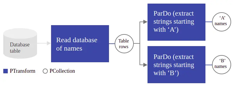
1. Pipeline: A Pipeline encapsulates your entire data processing task, from start to finish i.e. all the data and the transforms you perform on the data. All Beam driver programs must create a Pipeline.
2. PCollection: A PCollection represents a distributed data set that your Beam pipeline operates on. The data set can be discrete as well as continuous depending on whether your pipeline is a batch or a streaming one respectively. You can consider PCollections as the inputs and outputs for each step in your pipeline.
3. PTransform: A PTransform is a data processing operation, or a step, in your pipeline. Just as every function takes in some input, performs operations on that input and produces some output, every PTransform takes PCollection objects as input, performs a processing function that you provide on the elements of that PCollection, and produces zero or more output PCollection objects. You can use some existing Beam PTransform or write your own transforms depending on your use cases.

Hands-on

Now let's implement these concepts by writing our very own pipeline. Write a simple pipeline to process on a list of elements and print the results of our processing.

We will be using Python as the language of our choice. The Python SDK supports Python 3.7, 3.8, 3.9, 3.10, and 3.11. Apache Beam also provides support for other languages such as Java, Go, TypeScript.

Let's begin by installing the Apache Beam SDK if not already installed. To install it simply run the following in your terminal -

pip install apache-beam

Next import the modules required by our pipeline script.

import apache_beam as beam
import numpy as np # For creating arandom integer list.
import typing as t # For providing runtime supportfor type hints.

Let's initialize some data to work with. We will be creating a list having 100000 random integers from 0 to 5.

NUMBER_OF_ELEMENTS = 100000 # Creating a list of 100 thousandelements.
rand_int_list = np.random.randint(5, size=(NUMBER_OF_ELEMENTS))

A beam program often starts by creating a Pipeline object. We can do this by simply declaring a Pipeline object as context manager.

with beam.Pipeline() as p:
    pass # Build your pipeline here.

We will build our pipeline one step at a time.

First let's create some input data for our pipeline to work on.

• Create a PCollection which will serve as an input for our pipeline.
• We will use a beam source transform Create to create a PCollection.
• Simply pass in our random integer list to the transform to create a PCollection.

with beam.Pipeline() as p: 
    (
        p
        | "CreateValues" >> beam.Create(rand_int_list)
    )

| is a beam operator which applies a PTransform to a PCollection.

>> allows you to name a step in your pipeline. Names of the transform steps should be unique.

Our next step is to write some PTransforms to carry out our desired processing. We will be doing these following simple operations on the data.

1. Filter out the zero values from the data,
2. Perform simple arithmetic operations on the list values.

Each of these operations will be a separate step in our pipeline.

Operation 1: Filtering out elements

Apache beam provides a source transform called Filter to filter out the elements which don't satisfy the constraint condition. This transform will take in our custom function which will remove zero elements from the input PCollection.

Let's write a simple function to return values only if they are non-zero.

def simpleFilterFn(val: np.int64) -> np.int64:
    if val != 0:
        return val
    else:
        print("Skipping zero values...")

Now we will integrate the filter logic in our pipeline.

with beam.Pipeline() as p:
    (
        p
        | "CreateValues" >> beam.Create(rand_int_list) 
        | "FilterValues" >> beam.Filter(simpleFilterFn)
    )

Operation 2: Performing some arithmetic calculations on the data

We will make use of beam.ParDo core transform which allows us to specify custom processing functions to the elements of PCollections. ParDo simply stands for "parallel do".

We create custom PTransforms by using the beam.DoFn base class. Let's create classes for these transform operations.

class simpleDoFn(beam.DoFn):
    def _user_defined_function(self,data: np.int64) -> np.int64:
        # This will simply yield the data elementas it is.
        # You can change the transform logic here accordingly.
        return (data ** 2) / data

    def process(self, val: np.int64) -> t.Iterator[np.int64]:
        yield self._user_defined_function(val)

The process method is called for each element in the input PCollection, and it allows you to transform, filter, or perform any other operation on the data.

Note: We could also have alternatively written our filter logic in a beam.DoFn base class -

# The filter transform class.
class simpleFilter(beam.DoFn):
    def process(self, val: np.int64) -> t.Iterator[np.int64]:
        if val != 0:
            yield val
        else: print("Skipping zero values...")

Now that we have written the logic, let's integrate these transforms into our pipeline.

with beam.Pipeline() as p:
    (
        p
        | "CreateValues" >> beam.Create(rand_int_list)
        | "FilterValues" >> beam.Filter(simpleFilterFn)
        | "ProccessValues" >> beam.ParDo(simpleDoFn())
    )

And there you have it lads! You have successfully written your pipeline. You can apply a beam.Map transform to print out your result PCollection elements.

with beam.Pipeline() as p:
    (
        p
        | "CreateValues" >> beam.Create(rand_int_list)
        | "FilterValues" >> beam.Filter(simpleFilterFn)
        | "ProccessValues" >> beam.ParDo(simpleDoFn())
        | "PrintValues" >> beam.Map(print)
    )

Note: If you don't prefer using a context manager, the following will work as well -

p = beam.Pipeline()
vals = p | "CreateValues" >> beam.Create(rand_int_list)
filtered_vals = vals | "FilterValues" >> beam.Filter(simpleFilterFn)
processed_vals = filtered_vals | "ProccessValues" >> beam.ParDo(simpleDoFn())
_ = processed_vals | "PrintValues" >> beam.Map(print)
p.run()

Running the pipeline

To run the pipeline, simply execute the python script. By default the DirectRunner is chosen and this will execute the pipeline using your local machine resources. This approach is great for testing and debugging your pipelines before deploying them.

Beam also provides a number of runners to execute our pipelines on their resources. A runner runs your pipeline on the specified data processing system. The available runners include DirectRunner (local machine), DataFlowRunner, FlinkRunner, SparkRunner, SamzaRunner, NemoRunner.

Bonus

Wow! If you are still here, let's try to implement two more operations for our data.

We will find the average and standard deviation of our elements. Calculating these is a bit different than our previous operations.

Now, we all know how to calculate the mean of N number of elements i.e. (sum of the N elements)/N. That is easy when we have all the data present with us. But, in the case of Beam the data may be distributed across multiple worker machines. So the natural thing to do is to combine all the elements first, then calculate their mean.

We will be making use of another Beam core transform called CombineGlobally to aggregate the elements across the PCollection. We have to pass in our custom transformation logic to this transform which we will do by creating our own beam.CombineFn class (similar to creating a beam.DoFn class for the ParDo transform).

A general combining operation consists of four operations. When you create a subclass of CombineFn, you must provide four operations by overriding the corresponding methods:

1. Create Accumulator for initializing a new "local" accumulator.
2. Add Input adds an input element to an accumulator, returning the accumulator value.
3. Merge Accumulators merges several accumulators into a single accumulator; this is how data in multiple accumulators is combined before the final calculation.
4. Extract Output performs the final computation.

For calculating the mean, we will need to keep track of 2 things - sum of elements and the count of elements. Let's define our combiner class.

class MeanFn(beam.CombineFn):
    def create_accumulator(self) -> t.Tuple[float, int]:
        # Initialize the sum and count accumulators.
        return (0.0, 0)

    def add_input(self, sum_count, input_element) -> t.Tuple[float, int]:
        # Accumulates the sum of values and increments
        # the count as elementsare added.
        (sum, count) = sum_count
        return sum + input_element, count + 1

    def merge_accumulators(self, accumulators) -> t.Tuple[float, int]:
        # Combines multiple accumulators by summing their
        # sums and counts.
        total_sum = sum(acc[0] for acc in accumulators)
        total_count = sum(acc[1] for acc in accumulators)
        return (total_sum, total_count)

    def extract_output(self, sum_count) -> float:
        # Calculates the mean by dividing the sum by the count.
        (sum, count) = sum_count
        # Handles the case where the count is zero.
        return sum / count if count else float('NaN')

Now let's integrate this combiner logic in our pipeline.

with beam.Pipeline() as p:
    (
        p
        | "CreateValues" >> beam.Create(rand_int_list)
        | "FilterValues" >> beam.Filter(simpleFilterFn)
        | "ProccessValues" >> beam.ParDo(simpleDoFn())
        | "AverageValues" >> beam.CombineGlobally(MeanFn())
        | "PrintMean" >> beam.Map(print)
    )

Similarly for calculating the standard deviation we will need to keep track of three things - the sum of elements, the sum of the squares of elements and the count of elements. Remember this formula for standard deviation from high school -

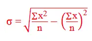
The latter part is nothing but the square of the mean. Let's define the combiner class.

class StdDevCombineFn(beam.CombineFn):
    def create_accumulator(self) -> t.Tuple[float, float, int]:
        # Initialize the accumulator as a tuple
        # (sum, sum_of_squares, count)
        return (0.0, 0.0, 0)

    def add_input(self, accumulator, input_element) -> t.Tuple[float, float, int]: 
        sum_values, sum_of_squares, count = accumulator
        input_value = float(input_element)
        return (sum_values + input_value, sum_of_squares + input_value ** 2, count + 1)

    def merge_accumulators(self, accumulators) -> t.Tuple[float, float, int]:
        total_sum = sum(acc[0] for acc in accumulators)
        total_sum_of_squares = sum(acc[1] for acc in accumulators)
        total_count = sum(acc[2] for acc in accumulators)
        return (total_sum, total_sum_of_squares, total_count)

    def extract_output(self, accumulator) -> float:
        sum_values, sum_of_squares, count = accumulator
        # Avoid division by zero.
        if count == 0:
            return 0.0
        mean = sum_values / count
        variance = (sum_of_squares / count) - (mean ** 2)
        # Avoid negative variance due to floating-point precision.
        if variance < 0:
            variance = 0.0
        return math.sqrt(variance)

You can also find other useful Beam source transforms for your use cases.

Conclusion

These simple pipelines barely tap into a small fraction of the enormous powerhouse of Apache Beam. But now that you know the in and outs of Beam and have the foundation built, you can write more advanced and complex pipelines.

References

• https://beam.apache.org/